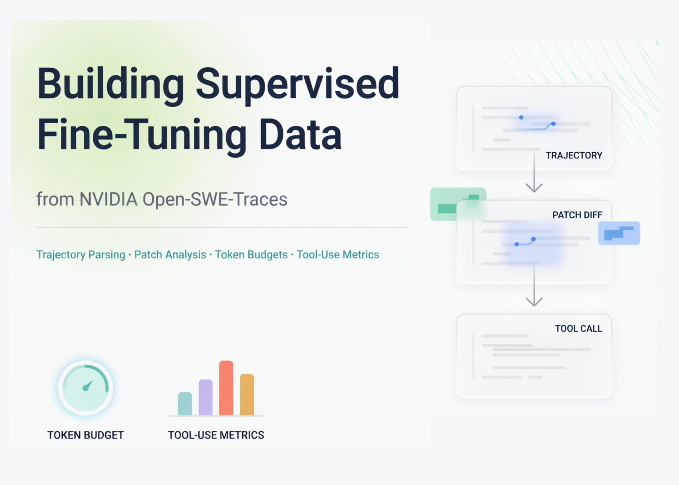
In this tutorial, we explore the Open-SWE-Traces dataset as a practical resource for studying and preparing agentic software-engineering trajectories for fine-tuning. We stream the dataset directly from Hugging Face, so we can work with a large dataset efficiently in Google Colab without downloading everything locally. We inspect individual records, normalize multi-turn agent conversations, parse final code patches, extract useful metadata, and build an analysis DataFrame to understand trajectory length, tool usage, patch size, language distribution, and resolution outcomes. We then use these insights to create a curated supervised fine-tuning subset that keeps only high-quality trajectories based on success labels, token limits, language filters, and patch availability.
Installing Dependencies and Configuration
import subprocess, sys def _pip(*pkgs): subprocess.run([sys.executable, "-m", "pip", "install", "-q", *pkgs], check=False) _pip("-U", "datasets", "huggingface_hub") _pip("tiktoken", "pandas", "matplotlib") import json import re import textwrap from itertools import islice from collections import Counter import pandas as pd import matplotlib.pyplot as plt from datasets import load_dataset pd.set_option("display.max_columns", 50) pd.set_option("display.width", 160) plt.rcParams.update({ "figure.figsize": (9, 4.6), "figure.dpi": 110, "axes.grid": True, "grid.alpha": 0.25, "axes.spines.top": False, "axes.spines.right": False, "font.size": 11, "axes.titlesize": 13, "axes.titleweight": "bold", }) BLUE, ORANGE, GREEN, RED = "#4C72B0", "#DD8452", "#55A868", "#C44E52" def banner(title): line = "=" * 78 print(f"n{line}n {title}n{line}") DATASET = "nvidia/Open-SWE-Traces" AGENTS = ["openhands", "sweagent"] MODELS = ["minimax_m25", "qwen35_122b"] SAMPLE_ALL = True PER_COMBO = 400 N_SINGLE = 1500 MAX_SFT_TOKENS = 32000 SFT_REQUIRE_RESOLVED = True SFT_LANGUAGES = None We start by installing and importing the core libraries needed for streaming, parsing, analysis, and visualization. We configure pandas and matplotlib to ensure our tables and plots remain readable in Google Colab. We also define the dataset name, agent/model combinations, sampling size, and SFT filtering settings that control the rest of the tutorial.
Defining Trajectory Parsing Helpers
def message_text(msg): if not isinstance(msg, dict): return "" content = msg.get("content", "") if content is None: return "" if isinstance(content, str): return content if isinstance(content, list): parts = [] for block in content: if isinstance(block, dict): parts.append(block.get("text") or block.get("content") or "") elif isinstance(block, str): parts.append(block) return "n".join(p for p in parts if p) return str(content) def normalize_trajectory(traj): if traj is None: return [] if isinstance(traj, str): try: traj = json.loads(traj) except Exception: return [] norm = [] for msg in traj: if isinstance(msg, str): try: msg = json.loads(msg) except Exception: msg = {"role": "unknown", "content": msg} if isinstance(msg, dict): norm.append(msg) return norm def normalize_metadata(meta): if isinstance(meta, str): try: return json.loads(meta) except Exception: return {} return meta if isinstance(meta, dict) else {} def role_counts(trajectory): c = Counter() for msg in trajectory or []: if isinstance(msg, dict): c[msg.get("role", "unknown")] += 1 return c _FUNC_XML = re.compile(r"", re.IGNORECASE) _BASH_FENCE = re.compile(r"```(?:bash|sh|shell)b", re.IGNORECASE) def extract_tool_names(trajectory): names = Counter() for msg in trajectory or []: if not isinstance(msg, dict): continue for call in msg.get("tool_calls") or []: fn = (call or {}).get("function", {}) if isinstance(call, dict) else {} if fn.get("name"): names[fn["name"]] += 1 if msg.get("role") == "tool" and msg.get("name"): names[msg["name"]] += 1 if msg.get("role") == "assistant": text = message_text(msg) for m in _FUNC_XML.findall(text): names[m.lower()] += 1 for m in _EXEC_TAG.findall(text): names[m.lower()] += 1 if _BASH_FENCE.search(text): names["bash_block"] += 1 return names def parse_patch(diff_text): if not diff_text or not isinstance(diff_text, str): return 0, 0, 0, [], Counter() files, exts = [], Counter() additions = deletions = 0 for line in diff_text.splitlines(): if line.startswith("diff --git"): parts = line.split() if len(parts) >= 3: path = parts[2][2:] if parts[2].startswith("a/") else parts[2] files.append(path) base = path.split("https://www.marktechpost.com/")[-1] if "." in base: exts[base.rsplit(".", 1)[-1].lower()] += 1 elif line.startswith("+") and not line.startswith("+++"): additions += 1 elif line.startswith("-") and not line.startswith("---"): deletions += 1 return len(files), additions, deletions, files, exts def make_token_counter(): try: import tiktoken enc = tiktoken.get_encoding("cl100k_base") return lambda s: len(enc.encode(s, disallowed_special=())) except Exception: return lambda s: max(1, len(s) // 4) count_tokens = make_token_counter() We define helper functions that make the dataset easier to process, even when fields appear in different formats. We normalize trajectories, extract message text, count roles, detect tool usage, parse code patches, and estimate token lengths. We build these utilities defensively so that our analysis remains stable across schema variations in large streamed datasets.
Streaming and Inspecting Trajectories
def stream_take(agent, model, n): ds = load_dataset(DATASET, agent, split=model, streaming=True) rows = [] for ex in islice(ds, n): ex = dict(ex) ex["_agent"], ex["_model"] = agent, model rows.append(ex) return rows banner("STEP 1 — Streaming trajectories from the Hub") raw_rows = [] if SAMPLE_ALL: combos = [(a, m) for a in AGENTS for m in MODELS] for agent, model in combos: try: part = stream_take(agent, model, PER_COMBO) raw_rows.extend(part) print(f" ✓ {agent:<10} / {model:<12} -> {len(part):>4} rows") except Exception as e: print(f" ✗ {agent}/{model} failed: {type(e).__name__}: {e}") else: raw_rows = stream_take(AGENTS[0], MODELS[0], N_SINGLE) print(f" ✓ {AGENTS[0]} / {MODELS[0]} -> {len(raw_rows)} rows") print(f"n Total rows pulled into memory: {len(raw_rows)}") assert raw_rows, "No rows streamed — check your internet connection and retry." banner("STEP 2 — Anatomy of a single record") sample = raw_rows[0] print("Top-level fields :", list(sample.keys())) print("instance_id :", sample.get("instance_id")) print("repo / language :", sample.get("repo"), "https://www.marktechpost.com/", sample.get("language")) print("license :", sample.get("license")) print("resolved (1/0/-1):", sample.get("resolved")) print("metadata :", normalize_metadata(sample.get("metadata"))) traj0 = normalize_trajectory(sample.get("trajectory")) print(f"nTrajectory has {len(traj0)} messages. Role histogram: {dict(role_counts(traj0))}") print("n--- Trajectory walkthrough (each message truncated to 240 chars) ---") for i, msg in enumerate(traj0[:8]): role = msg.get("role", "unknown").upper() body = " ".join(message_text(msg).split()) print(f"n[{i}] {role}") print(textwrap.fill(body[:240] + ("…" if len(body) > 240 else ""), width=92, subsequent_indent=" ")) if len(traj0) > 8: print(f"n… (+{len(traj0) - 8} more messages)") print("n--- Final patch (model_patch), first 25 lines ---") print("n".join((sample.get("model_patch") or "").splitlines()[:25]) or "(empty)") We stream a small sample of Open-SWE-Traces directly from Hugging Face instead of downloading the full dataset. We collect examples across agent and model combinations, then inspect the structure of a single record in detail. We walk through the first few trajectory messages and preview the final patch to understand what each training example contains.
Building the Analysis DataFrame
banner("STEP 3 — Building the analysis DataFrame") def process_example(ex): traj = normalize_trajectory(ex.get("trajectory")) rc = role_counts(traj) nf, add, dele, _files, _exts = parse_patch(ex.get("model_patch")) meta = normalize_metadata(ex.get("metadata")) full_text = "n".join(message_text(m) for m in traj) return { "instance_id": ex.get("instance_id"), "repo": ex.get("repo"), "language": (ex.get("language") or "unknown").lower(), "license": ex.get("license"), "resolved": ex.get("resolved"), "agent": ex.get("_agent"), "model": ex.get("_model"), "n_messages": len(traj), "n_system": rc.get("system", 0), "n_user": rc.get("user", 0), "n_assistant": rc.get("assistant", 0), "n_tool": rc.get("tool", 0), "patch_files": nf, "patch_add": add, "patch_del": dele, "patch_churn": add + dele, "traj_tokens": count_tokens(full_text), "category": meta.get("category"), "meta_files": meta.get("num_modified_files"), "meta_lines": meta.get("num_modified_lines"), "_tools": extract_tool_names(traj), } records = [process_example(ex) for ex in raw_rows] df = pd.DataFrame(records) df["is_resolved"] = (df["resolved"] == 1) df["known_label"] = df["resolved"].isin([0, 1]) print(f"DataFrame: {df.shape[0]} rows x {df.shape[1]} cols") print("nNumeric summary:") print(df[["n_messages", "n_assistant", "n_tool", "patch_files", "patch_churn", "traj_tokens"]].describe().round(1)) We transform the raw streamed records into a structured pandas DataFrame for analysis. We extract trajectory-level features such as message counts, role counts, patch churn, token estimates, metadata fields, and tool-use counters. We also create resolution flags to compare successful and unsuccessful software-engineering trajectories.
Visualizing Trajectory Distributions
banner("STEP 4 — Distributions & visualizations") lang_counts = df["language"].value_counts() print("Trajectories per language:n", lang_counts.to_string()) ax = lang_counts.plot(kind="bar", color=BLUE) ax.set_title("Trajectories per language (sample)") ax.set_xlabel(""); ax.set_ylabel("count") plt.tight_layout(); plt.show() known = df[df["known_label"]] by_lang = (known.groupby("language")["is_resolved"] .agg(rate="mean", n="size") .query("n >= 25") .sort_values("rate", ascending=False)) print("nResolution rate by language (n>=25):n", by_lang.round(3).to_string()) if not by_lang.empty: ax = by_lang["rate"].plot(kind="bar", color=GREEN) ax.set_title("Resolution rate by language") ax.set_xlabel(""); ax.set_ylabel("fraction resolved"); ax.set_ylim(0, 1) plt.tight_layout(); plt.show() if known["agent"].nunique() > 1 or known["model"].nunique() > 1: pivot = (known.groupby(["agent", "model"])["is_resolved"].mean().unstack()) print("nResolution rate by scaffold x model:n", pivot.round(3).to_string()) ax = pivot.plot(kind="bar", color=[BLUE, ORANGE]) ax.set_title("Resolution rate: scaffold x model") ax.set_xlabel("agent"); ax.set_ylabel("fraction resolved"); ax.set_ylim(0, 1) ax.legend(title="model"); plt.tight_layout(); plt.show() ax = df["n_messages"].plot(kind="hist", bins=40, color=BLUE, alpha=0.85) ax.set_title("Messages per trajectory") ax.set_xlabel("number of messages"); ax.set_ylabel("trajectories") plt.tight_layout(); plt.show() churn = df["patch_churn"].clip(upper=df["patch_churn"].quantile(0.97)) ax = churn.plot(kind="hist", bins=40, color=ORANGE, alpha=0.85) ax.set_title("Patch size — lines changed (clipped at p97)") ax.set_xlabel("added + deleted lines"); ax.set_ylabel("trajectories") plt.tight_layout(); plt.show() if known["is_resolved"].nunique() > 1: fig, ax = plt.subplots() for flag, color, lab in [(True, GREEN, "resolved"), (False, RED, "unresolved")]: sub = known[known["is_resolved"] == flag] ax.scatter(sub["n_messages"], sub["traj_tokens"], s=10, alpha=0.4, color=color, label=lab) ax.set_title("Trajectory length vs. token size, by outcome") ax.set_xlabel("messages"); ax.set_ylabel("estimated tokens") ax.legend(); plt.tight_layout(); plt.show() Analyzing Token Budget Requirements
banner("STEP 5 — Token budget (what context window do you need?)") tok = df["traj_tokens"] print("Estimated tokens per trajectory — percentiles:") for p in [50, 75, 90, 95, 99]: print(f" p{p:<2}: {int(tok.quantile(p/100)):>8,}") print(f" max: {int(tok.max()):>8,}") windows = [8_192, 16_384, 32_768, 65_536, 131_072] print("nFraction of trajectories that fit in a given context window:") for w in windows: frac = (tok <= w).mean() print(f" {w:>7,} tokens : {frac*100:5.1f}%") ax = tok.clip(upper=tok.quantile(0.99)).plot(kind="hist", bins=50, color=BLUE, alpha=0.85) for w, c in zip([8_192, 32_768, 131_072], [GREEN, ORANGE, RED]): if w <= tok.quantile(0.99): ax.axvline(w, color=c, ls="--", lw=1.5, label=f"{w//1024}k ctx") ax.set_title("Trajectory token-length distribution (clipped at p99)") ax.set_xlabel("estimated tokens"); ax.set_ylabel("trajectories") ax.legend(); plt.tight_layout(); plt.show() banner("STEP 6 — Which tools/actions do the agents use?") tool_totals = Counter() for t in df["_tools"]: tool_totals.update(t) top_tools = tool_totals.most_common(12) if top_tools: print("Most frequent agent actions (across the sample):") for name, cnt in top_tools: print(f" {name:<24} {cnt:>7,}") labels, vals = zip(*top_tools) fig, ax = plt.subplots(figsize=(9, 5)) ax.barh(range(len(labels)), vals, color=BLUE) ax.set_yticks(range(len(labels))); ax.set_yticklabels(labels) ax.invert_yaxis() ax.set_title("Top agent actions / tool invocations") ax.set_xlabel("count"); plt.tight_layout(); plt.show() else: print("No tool actions detected with the current heuristics.") if known["is_resolved"].nunique() > 1: print("nMean 'tool' (environment) turns by outcome:") print(known.groupby("is_resolved")["n_tool"].mean().round(2).to_string()) We explore the dataset through language counts, resolution rates, scaffold/model comparisons, message-length distributions, patch-size distributions, and token-budget analysis. We visualize how trajectory length, token size, and tool usage vary across the sampled records. We use these plots and summaries to determine which examples are practical to fine-tune under different context-window limits.
Building a Curated SFT Subset
banner("STEP 7 — Building a curated SFT subset") def to_chatml(trajectory): out = [] for m in trajectory: role = m.get("role", "unknown") out.append(f"<|im_start|>{role}n{message_text(m).strip()}<|im_end|>") return "n".join(out) def passes_filters(rec, raw): if SFT_REQUIRE_RESOLVED and rec["resolved"] != 1: return False if rec["traj_tokens"] > MAX_SFT_TOKENS: return False if SFT_LANGUAGES is not None and rec["language"] not in SFT_LANGUAGES: return False if not (raw.get("model_patch") or "").strip(): return False return True sft_examples = [] for rec, raw in zip(records, raw_rows): if not passes_filters(rec, raw): continue messages = [{"role": m.get("role"), "content": message_text(m)} for m in normalize_trajectory(raw.get("trajectory"))] sft_examples.append({ "instance_id": rec["instance_id"], "repo": rec["repo"], "language": rec["language"], "agent": rec["agent"], "model": rec["model"], "messages": messages, "text": to_chatml(messages), "model_patch": raw.get("model_patch"), "approx_tokens": rec["traj_tokens"], }) print(f"Kept {len(sft_examples)} / {len(records)} trajectories after filtering") print(f" filters -> resolved_only={SFT_REQUIRE_RESOLVED}, " f"max_tokens={MAX_SFT_TOKENS:,}, languages={SFT_LANGUAGES or 'all'}") if sft_examples: kept = pd.DataFrame(sft_examples) print("nCurated subset by language:n", kept["language"].value_counts().to_string()) print("n--- One formatted SFT example (ChatML, truncated) ---") print(sft_examples[0]["text"][:600], "…") banner("STEP 8 — Exporting artifacts") csv_path = "open_swe_traces_analysis.csv" df.drop(columns=["_tools"]).to_csv(csv_path, index=False) print(f" Wrote analysis table -> {csv_path} ({len(df)} rows)") jsonl_path = "open_swe_sft.jsonl" with open(jsonl_path, "w", encoding="utf-8") as f: for ex in sft_examples: f.write(json.dumps(ex, ensure_ascii=False) + "n") print(f" Wrote SFT dataset -> {jsonl_path} ({len(sft_examples)} rows)") print("nDone. In Colab, open the Files pane (folder icon, left) to download both.") print("To load the SFT file later: datasets.load_dataset('json', " "data_files='open_swe_sft.jsonl')") We convert selected trajectories into an SFT-ready format using standardized message dictionaries and an optional ChatML-style text representation. We filter examples by resolution status, token budget, language selection, and patch availability to keep the curated subset useful for training. We finally export both the analysis CSV and the JSONL SFT dataset for reuse in later fine-tuning workflows.
Conclusion
In conclusion, we built a complete workflow to transform Open-SWE-Traces from a large, raw, agentic dataset into structured analytics and SFT-ready training data. We learned how to stream trajectories, inspect agent behavior, measure token budgets, compare scaffolds and models, analyze patch characteristics, and export both an analysis table and a JSONL training file. We now have a reusable framework that we can extend for larger sampling, language-specific fine-tuning, deeper tool-use analysis, and model-specific chat-template formatting.
Check out the Full Codes here. Also, feel free to follow us on Twitter and don’t forget to join our 150k+ML SubReddit and Subscribe to our Newsletter. Wait! are you on telegram? now you can join us on telegram as well.
Need to partner with us for promoting your GitHub Repo OR Hugging Face Page OR Product Release OR Webinar etc.? Connect with us

Sana Hassan
Sana Hassan, a consulting intern at Marktechpost and dual-degree student at IIT Madras, is passionate about applying technology and AI to address real-world challenges. With a keen interest in solving practical problems, he brings a fresh perspective to the intersection of AI and real-life solutions.